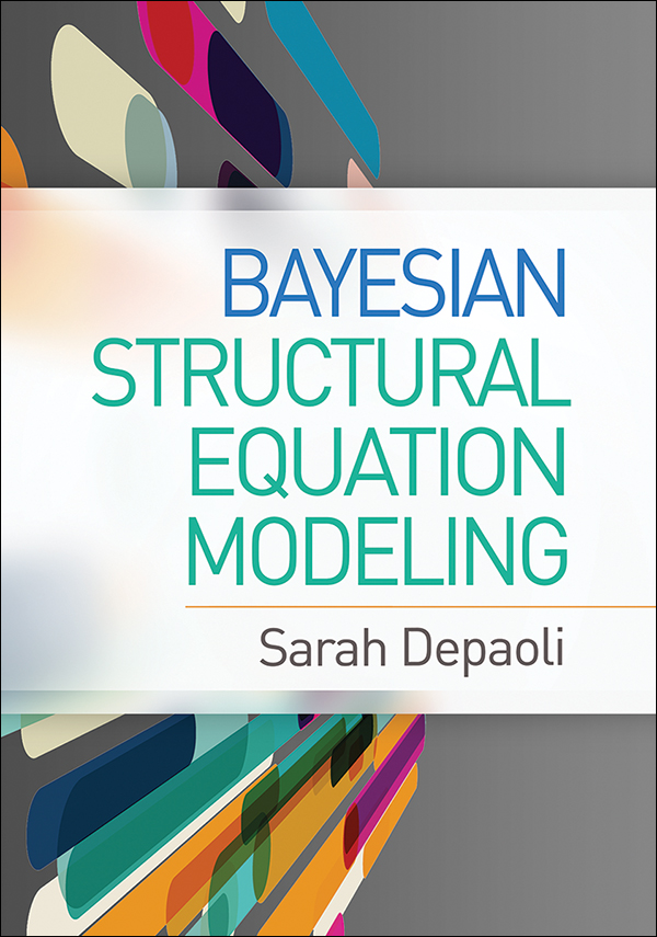
Bayesian Structural Equation Modeling

I. Introduction

1. Background

1.1. Bayesian Statistical Modeling: The Frequency of Use

1.2. The Key Impediments within Bayesian Statistics

1.3. Benefits of Bayesian Statistics within SEM

1.3.1. A Recap: Why Bayesian SEM?

1.4. Mastering the SEM Basics: Precursors to Bayesian SEM

1.4.1. The Fundamentals of SEM Diagrams and Terminology

1.4.2. LISREL Notation

1.4.3. Additional Comments about Notation

1.5. Datasets used in the Chapter Examples

1.5.1. Cynicism Data

1.5.2. Early Childhood Longitudinal Survey–Kindergarten Class

1.5.3. Holzinger and Swineford (1939)

1.5.4. IPIP 50: Big Questionnaire

1.5.5. Lakaev Academic Stress Response Scale

1.5.6. Political Democracy

1.5.7. Program for International Student Assessment

1.5.8. Youth Risk Behavior Survey

2. Basic Elements of Bayesian Statistics

2.1. A Brief Introduction to Bayesian Statistics

2.2. Setting the Stage

2.3. Comparing Frequentist and Bayesian Inference

2.4. The Bayesian Research Circle

2.5. Bayes’ Rule

2.6. Prior Distributions

2.6.1. The Normal Prior

2.6.2. The Uniform Prior

2.6.3. The Inverse Gamma Prior

2.6.4. The Gamma Prior

2.6.5. The Inverse Wishart Prior

2.6.6. The Wishart Prior

2.6.7. The Beta Prior

2.6.8. The Dirichlet Prior

2.6.9. Different Levels of Informativeness for Prior Distributions

2.6.10. Prior Elicitation

2.6.11. Prior Predictive Checking

2.7. The Likelihood (Frequentist and Bayesian Perspectives)

2.8. The Posterior

2.8.1. An Introduction to Markov Chain Monte Carlo Methods

2.8.2. Sampling Algorithms

2.8.3. Convergence

2.8.4. MCMC Burn-in Phase

2.8.5. The Number of Markov Chains

2.8.6. A Note about Starting Values

2.8.7. Thinning a Chain

2.9. Posterior Inference

2.9.1. Posterior Summary Statistics

2.9.2. Intervals

2.9.3. Effective Sample Size

2.9.4. Trace-plots

2.9.5. Autocorrelation Plots

2.9.6. Posterior Histogram and Density Plots

2.9.7. HDI Histogram and Density Plots

2.9.8. Model Assessment

2.9.9. Sensitivity Analysis

2.10. A Simple Example

2.11. Chapter Summary

2.11.1. Major Take Home Points

2.11.2. Notation Referenced

2.11.3. Annotated Bibliography of Select Resources

Appendix A: Getting Started with R

II. Measurement Models and Related Issues

3. The Confirmatory Factor Analysis Model

3.1. Introduction to Bayesian CFA

3.2. The Model and Notation

3.2.1. Handling Indeterminacies in CFA

3.3. The Bayesian Form of the CFA Model

3.3.1. Additional Information about the (Inverse) Wishart Prior

3.3.2. Alternative Priors for Covariance Matrices

3.3.3. Alternative Priors for Variances

3.3.4. Alternative Priors for Factor Loadings

3.4. Example: Basic Confirmatory Factor Analysis Model

3.5. Example: Implementing Near-Zero Priors for Cross-Loadings

3.6. How to Write up Bayesian CFA Results

3.6.1. Hypothetical Data Analysis Plan

3.6.2. Hypothetical Results Section

3.6.3. Discussion Points Relevant to the Analysis

3.7. Chapter Summary

3.7.1. Major Take Home Points

3.7.2. Notation Referenced

3.7.3. Annotated Bibliography of Select Resources

3.7.4. Example Code for Mplus

3.7.5. Example Code for R

4. Multiple Group Models

4.1. A Brief Introduction to Multi-Group Models

4.2. Introduction to the Multiple-Group CFA Model (with Mean Differences)

4.3. The Model and Notation

4.4. The Bayesian Form of the Multiple-Group CFA Model

4.5. Example: Using a Mean Differences, Multiple-Group CFA Model to Assess for School Differences

4.6. Introduction to the MIMIC Model

4.7. The Model and Notation

4.8. The Bayesian Form of the MIMIC Model

4.9. Example: Using the MIMIC Model to Assess for School Differences

4.10. How to Write up Bayesian Multiple-Group Model Results with Mean Differences

4.10.1. Hypothetical Data Analysis Plan

4.10.2. Hypothetical Results Section

4.10.3. Discussion Points Relevant to the Analysis

4.11. Chapter Summary

4.11.1. Major Take Home Points

4.11.2. Notation Referenced

4.11.3. Annotated Bibliography of Select Resources

4.11.4. Example Code for Mplus

4.11.5. Example Code for R

5. Measurement Invariance Testing

5.1. A Brief Introduction to Measurement Invariance in SEM

5.1.1. Stages of Traditional MI Testing

5.1.2. Challenges Within Traditional MI Testing

5.2. Bayesian Approximate MI

5.3. The Model and Notation

5.4. Priors within Bayesian Approximate MI

5.5. Example: Illustrating Bayesian Approximate MI for School Differences

5.5.1. Results for the Conventional MI Tests

5.5.2. Results for the Bayesian Approximate MI Tests

5.5.3. Results Comparing Latent Means Across Approaches

5.5.4. Hypothetical Data Analysis Plan

5.6. How to Write up Bayesian Approximate Measurement Invariance Results

5.6.1. Analytic Procedure

5.6.2. Results

5.6.3. Discussion Points Relevant to the Analysis

5.7. Chapter Summary

5.7.1. Major Take Home Points

5.7.2. Notation Referenced

5.7.3. Annotated Bibliography of Select Resources

5.7.4. Example Code for Mplus

5.7.5. Example Code for R

III. Extending the Structural Model

6. The General Structural Equation Model

6.1. Introduction to Bayesian SEM

6.2. The Model and Notation

6.3. The Bayesian form of SEM

6.4. Example: Revisiting Bollen’s (1989) Political Democracy Example

6.4.1. Motivation for this Example

6.4.2. The Current Example

6.5. How to Write up Bayesian SEM Results

6.5.1. Hypothetical Data Analysis Plan

6.5.2. Hypothetical Results Section

6.5.3. Discussion Points Relevant to the Analysis

6.6. Chapter Summary

6.6.1. Major Take Home Points

6.6.2. Notation Referenced

6.6.3. Annotated Bibliography of Select Resources

6.6.4. Example Code for Mplus

6.6.5. Example Code for R

Appendix A: Causal Inference and Mediation Analysis

7. Multilevel Structural Equation Modeling

7.1. Introduction to Multilevel SEM

7.1.1. MSEM Applications

7.1.2. Contextual Effects

7.2. Extending MSEM into the Bayesian Context

7.3. The Model and Notation

7.4. The Bayesian form of MSEM

7.5. Example: A 2-Level CFA with Continuous Items

7.5.1. Implementation of Example

7.5.2. Example Results

7.6. Example: A Three-Level CFA with Categorical Items

7.6.1. Implementation of Example

7.6.2. Example Results

7.7. How to Write up Bayesian MSEM Results

7.7.1. Hypothetical Data Analysis Plan

7.7.2. Hypothetical Results Section

7.7.3. Discussion Points Relevant to the Analysis

7.8. Chapter Summary

7.8.1. Major Take Home Points

7.8.2. Notation Referenced

7.8.3. Annotated Bibliography of Select Resources

7.8.4. Example Code for Mplus

7.8.5. Example Code for R

IV. Longitudinal and Mixture Models

8. Latent Growth Curve Modeling

8.1. Introduction to Bayesian LGCM

8.2. The Model and Notation

8.2.1. Extensions of the LGCM

8.3. The Bayesian Form of the LGCM

8.3.1. Alternative Priors for the Factor Variances and Covariances

8.4. Example: Bayesian Estimation of the LGCM using ECLS–K Reading Data

8.5. Example: Extending the Example to Include Separation Strategy Priors

8.6. Example: Extending the Framework to Assessing Measurement Invariance Over Time

8.7. How to Write up Bayesian LGCM Results

8.7.1. Hypothetical Data Analysis Plan

8.7.2. Hypothetical Results Section

8.7.3. Discussion Points Relevant to the Analysis

8.8. Chapter Summary

8.8.1. Major Take Home Points

8.8.2. Notation Referenced

8.8.3. Annotated Bibliography of Select Resources

8.8.4. Example Code for Mplus

8.8.5. Example Code for R

9. The Latent Class Model

9.1. A Brief Introduction to Mixture Models

9.2. Introduction to Bayesian LCA

9.3. The Model and Notation

9.3.1. Introducing the Issue of Class Separation

9.4. The Bayesian Form of the LCA Model

9.4.1. Adding Flexibility to the LCA Model

9.5. Mixture Models, Label Switching, and Possible Solutions

9.5.1. Identifiability Constraints

9.5.2. Relabeling Algorithms

9.5.3. Label Invariant Loss Functions

9.5.4. Final Thoughts on Label Switching

9.6. Example: A Demonstration of Bayesian LCA

9.6.1. Motivation for this Example

9.6.2. The Current Example

9.7. How to Write up Bayesian LCA Results

9.7.1. Hypothetical Data Analysis Plan

9.7.2. Hypothetical Results Section

9.7.3. Discussion Points Relevant to the Analysis

9.8. Chapter Summary

9.8.1. Major Take Home Points

9.8.2. Notation Referenced

9.8.3. Annotated Bibliography of Select Resources

9.8.4. Example Code for Mplus

9.8.5. Example Code for R

10. The Latent Growth Mixture Model

10.1. Introduction to Bayesian LGMM

10.2. The Model and Notation

10.2.1. Concerns with Class Separation

10.3. The Bayesian Form of the LGMM

10.3.1. Alternative Priors for Factor Means

10.3.2. Alternative Priors for the Measurement Error Covariance Matrix

10.3.3. Alternative Priors for the Factor Covariance Matrix

10.3.4. Handling Label Switching in LGMMs

10.4. Example: Comparing Different Prior Conditions in an LGMM

10.4.1. Hypothetical Data Analysis Plan

10.5. How to Write up Bayesian LGMM Results

10.5.1. Hypothetical Results Section

10.5.2. Discussion Points Relevant to the Analysis

10.6. Chapter Summary

10.6.1. Major Take Home Points

10.6.2. Notation Referenced

10.6.3. Annotated Bibliography of Select Resources

10.6.4. Example Code for Mplus

10.6.5. Example Code for R

V. Special Topics

11. Model Assessment

11.1. Model Comparison and Cross Validation

11.1.1. Bayes Factors

11.1.2. The Bayesian Information Criterion

11.1.3. The Deviance Information Criterion

11.1.4. The Widely Applicable Information Criterion

11.1.5. Leave-One-Out Cross-Validation

11.2. Model Fit

11.2.1. Posterior Predictive Model Checking

11.2.2. Missing Data and the PPC Procedure

11.2.3. Testing Near-Zero Parameters Through the PPPP

11.3. Bayesian Approximate Fit

11.3.1. Bayesian Root Mean Square Error of Approximation

11.3.2. Bayesian Tucker-Lewis Index

11.3.3. Bayesian Normed Fit Index

11.3.4. Bayesian Comparative Fit Index

11.3.5. Implementation of These Indices

11.4. Example: Illustrating the PPC and the PPPP for CFA

11.5. Example: Illustrating Bayesian Approximate Fit for CFA

11.6. How to Write up Bayesian Approximate Fit Results

11.6.1. Hypothetical Data Analysis Plan

11.6.2. Hypothetical Results Section

11.6.3. Discussion Points Relevant to the Analysis

11.7. Chapter Summary

11.7.1. Major Take Home Points

11.7.2. Notation Referenced

11.7.3. Annotated Bibliography of Select Resources

11.7.4. Example Code for Mplus

11.7.5. Example Code for R

12. Important Points to Consider

12.1. Implementation and Reporting of Bayesian Results

12.1.1. Priors Implemented

12.1.2. Convergence

12.1.3. Sensitivity Analysis

12.1.4. How Should We Interpret These Findings?

12.2. Points to Check Prior to Data Analysis

12.2.1. Is Your Model Formulated “Correctly”?

12.2.2. Do You Understand the Priors?

12.3. Points to Check After Initial Data Analysis, but Before Interpretation of Results

12.3.1. Convergence

12.3.2. Does Convergence Remain After Doubling the Number of Iterations?

12.3.3. Is There Ample Information in the Posterior Histogram?

12.3.4. Is There a Strong Degree of Autocorrelation in the Posterior?

12.3.5. Does the Posterior make Substantive Sense?

12.4. Understanding the Influence of Priors

12.4.1. Examining the Influence of Priors on Multivariate Parameters (e.g., Covariance Matrices)

12.4.2. Comparing the Original Prior to Other Diffuse or Subjective Priors

12.5. Incorporating Model Fit or Model Comparison

12.6. Interpreting Model Results the “Bayesian Way”

12.7. How to Write up Bayesian Results

12.7.1. (Hypothetical) Results for Bayesian Two-Factor CFA

12.8. How to Review Bayesian Work

12.9. Chapter Summary and Looking Forward

References

Glossary

About the Author